Clinical Epidemiology and Biostatistics
An ability to read the medical literature intelligently is an essential skill for the competent clinical practitioner. Acquiring this skill is challenging because of the high volume of medical articles published and the increasing sophistication of modern epidemiologic and statistical methods.
Topics that will be covered in this chapter include:
1. Exposures and outcomes
2. Types of clinical studies
3. Types of statistical errors
4. Data presentation: reporting of outcomes
5. Confounding and interaction
6. Multivariable regression and pitfalls
7. Bias and its consequences
8. External validity: assessments of causation and validity
9. Issues related to:
a. Randomized treatment/prevention trials
b. Studies of diagnostic tests
c. Prognostic (survival) studies
d. Case–control studies
e. Economics
f. Clinical prediction guides
g. Systematic review articles and meta-analyses
CURRENT CONCEPTS AND ESSENTIAL FACTS
Exposures and Outcomes
At the heart of virtually all clinical studies is an attempt to link an “exposure” with an “outcome.” When reading an article, you should ask yourself what exactly the exposure and outcome variables are and whether their association is of interest to you.
For exposure, the “independent” variable, examples include:
1. A treatment strategy (or lack thereof)
2. A patient characteristic (such as age, gender, or cholesterol level)
3. A diagnostic test result (such as ejection fraction)
For outcome, the “dependent” variable, examples include:
1. A treatment outcome (such as death, myocardial infarction, need for revascularization)
2. A clinical event during follow-up (such as death or myocardial infarction)
3. A “gold standard” finding (such as evidence of coronary disease on an angiogram)
Types of Clinical Studies
Various types of clinical studies are reported in the literature, including the following.
Case Reports
Case reports, although they may be fun to read, rarely provide the kind of high-level evidence needed to influence clinical practice.
Case Series
Case series report on a group of patients who show a certain finding. Although there may be a clear-cut exposure and an outcome variable, the absence of a comparison group limits any conclusions that can be drawn. Case reports and case series are best thought of as hypothesis-generating studies.
Cohort Study
The cohort study is a fundamentally strong study design in which:
1. An inception cohort is clearly defined.
2. An exposure variable is defined.
3. The cohort consists of individuals with and without the exposure variable present at the time of inception.
4. The cohort is followed over time for the occurrence of a clearly and objectively defined outcome.
5. The occurrence of the outcome is compared in individuals with and without the exposure variable.
Case–Control Study
A case–control study (Fig. 7.1) is a somewhat weaker study design than a cohort study. In a case–control study:
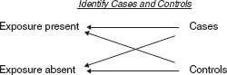
1. A “case” group of subjects with a given outcome is identified.
2. A “control” group of subjects, without the outcome, is identified.
3. The occurrence of an exposure variable is compared between the case group and the control group.
Studies of Diagnostic Tests
In studies designed to assess the value of a diagnostic test, a group of patients suspected of having a certain disease (outcome) undergo the diagnostic test, and then the results of the diagnostic test are compared against an accepted standard.
Cost-Effectiveness Studies
Cost-effectiveness studies usually take the form of a cohort study in which (a) the cost of an intervention is measured, (b) the outcomes of performing or not performing an intervention are compared, or (c) the cost of preventing an outcome is measured; typically, this last is recorded as dollars per year of life saved or dollars per quality-adjusted year of life saved (QALY).
Randomized Controlled Trials
Randomized controlled trials (Fig. 7.2) are the gold standard for assessing a treatment or a prevention measure. In these studies:
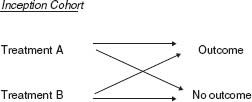
FIGURE 7.2 Randomized trial diagram.
1. A cohort of patients at risk for an outcome is defined.
2. Determination of which patients receive treatment or prevention is made entirely at random.
3. An outcome is measured after a predetermined follow-up period.
In effect, a randomized controlled trial is a kind of cohort study, except that the exposure variable is determined by the investigator, not by nature, using a randomization technique.
Prospective-versus-Retrospective Studies
In prospective-versus-retrospective studies, prospective data are obtained and coded at the time they are first available and, in the case of cohort studies, prior to the outcome. Retrospective data are obtained at a later time, often after the outcome has occurred.
Prospective studies are much less likely to be subject to observation bias or problems with missing data.
Meta-Analysis
Meta-analyses are systematic reviews of specific clinical questions with data pooled from multiple previously completed/published studies. Steps in a meta-analysis include:
1. Clinical hypothesis is defined.
2. Literature is searched.
3. Studies are selected based on prespecified criteria.
4. Consistent summary measures are collected from each identified study.
5. Pooled analysis is performed.
Most meta-analyses only pool randomized clinical trials, but meta-analyses can include cohort studies alone or mixed with clinical trials. Meta-analyses may suffer from publication bias as negative studies have traditionally been more difficult to publish.
Genome-Wide Association Studies
Genome-wide association studies (GWAS) are a contemporary form of case–control studies that focus on genetic data. DNA from people with (cases) and without (controls) a disease is collected and placed on gene chips. These chips are read into computers that identify DNA variations between the two groups . DNA variations that are more frequently detected are “associated” with the disease and hint at chromosomal regions that may be responsible for the disease.
Statistical Tests
Statistics is the science by which observations made of a sample are assessed with respect to their likely validity in the entire universe.
Type I and Type II Errors
Commonly reported statistics include two types of statistical error analysis. In type I errors, an association between an exposure and an outcome is in fact a spurious one that has resulted from random chance. The “p value” refers to the likelihood that an observed association is due to chance alone. In type II errors, on the other hand, the lack of an observed association between an exposure and an outcome is in fact due to chance because the sample size was not large enough to detect an association if one in fact exists. This is one of the most common errors reported in clinical literature.
Hypothesis Testing
Statistical tests also aim to determine whether a “null hypothesis” should be rejected, where the null hypothesis is that no association exists between the exposure and the outcome. Today many clinical researchers are moving away from this sort of hypothesis testing and more toward estimation of effects along with confidence intervals, discussed below.
Comparisons of Continuous Variables
Continuous variables are variables that can have an infinite number of values, such as age, height, blood pressure, or cholesterol level. They are described using means, standard deviations, ranges, quartiles, quintiles, deciles, and so on.
When continuous variables are normally distributed (i.e., described by a Gaussian or bell-shaped curve), t tests are generally used to compare the means of two groups and ANOVA is used to compare means of three or more groups.
When the continuous variables cannot be assumed to be normally distributed, nonparametric testing, such as the Wilcoxon rank-sum, which compares median values and distributions of two groups, or the Kruskal-Wallis test, which compares medians and distributions of three or more groups, is often used.
To compare the strength of a presumed linear association between two continuous variables (e.g., left ventricle mass versus blood pressure), researchers often use tests of correlation (r value), such as Pearson or Spearman tests. In these tests, the square of the r value describes how much the variability of one variable can be attributed to the other.
Comparisons of Categorical Variables
Variables that can only have a finite set of values (e.g., gender, presence or absence hypertension, use of a certain medication) are called categorical variables. For most samples, these kinds of variables are compared using the chi-square test. However, if the sample size is very small, researchers may instead use the Fischer exact test.
Data Presentation and Reporting of Outcomes
The statistical tests discussed above tell only part of the story. The strengths of associations can be described in a number of ways.
Number of Outcomes
Knowing the number of outcomes is essential to determining the strength of a study. In general, studies with <25 outcome occurrences are suspect. Studies with >100 outcomes may be compelling.
Absolute Event Rates
Absolute event rates are generally considered the most honest way to present data. How many outcomes were associated with exposures? How many outcomes occurred among those not exposed? Be suspicious if raw data are not provided. A careful reading of the raw data will enables a reader to distinguish between “statistical significance” and “clinical significance.” It is the latter that we really care about.
Relative Risk or Risk Ratio
Relative risk or risk ratio (RR) is the proportion of event rates according to exposure, or

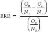
where OE is the number of patients with exposure who had the outcome. NE is the number of patients with exposure, O0 is the number of patients without exposure who had the outcome and N0 is the number of patients without exposure.
A risk ratio of 1.0 implies no association; a value >1 implies an increased risk, and a value <1 implies a protective effect.
Relative Risk Reduction
Relative risk reduction (RRR) is defined as the proportional reduction in rates, or
Absolute Risk Reduction
Absolute risk reduction (ARR) is the difference between absolute event rates, a more honest way of presenting data, or

Number Needed to Treat
Number needed to treat (NNT) is the number of patients who would need to be exposed in order to prevent one outcome, or

Confidence Interval
The confidence interval (CI) is a measure of uncertainty; given a 95% confidence interval, we can be 95% sure that the true measure lies somewhere within the interval.
Odds are another way of describing the frequency of an event. For any given population in which O outcomes occur among N subjects,

In effect, this is the probability of an event occurring divided by the probability that the event will not occur. The odds ratio compares odds between exposed and unexposed groups.
It is very important that you not confuse odds ratios with risk ratios (or relative risks). Generally, odds ratios and risk ratios are similar only if the outcome event rates are low (i.e., <10%).
Hazard Ratio
The hazard ratio is used specifically in survival studies. The hazard is the instantaneous probability of an event occurring given that a subject has survived for a certain period of time without experiencing that event. The hazard ratio compares the hazards of exposed and unexposed groups.
Attributable Risk
Attributable risk measures the relative contribution of a given exposure to an outcome in a population. Thus, if we assume that the association is causal and we then remove the exposure, the attributable risk tells us by how much the outcome event rate should be reduced. Attributable risk (AR) is calculated as

where P is the prevalence of exposure (or NE/[NE+ N0]) and RR is the relative risk as described above.
Kaplan–Meier Event Rates
Kaplan–Absolute risk reduction Meier event rates are a graphical way of showing time free of an event. This method takes into account variable follow-up times (or censoring), an issue that is common in studies of outcomes of chronic diseases.
An example showing how these terms are calculated is now shown. Imagine a clinical trial in which 10,000 patients are randomized in a 1:1 manner to either drug A or drug B (i.e., 5,000 are assigned drug A and 5,000 are assigned drug B). Suppose that 2,500 of the drug A patients experience events, whereas 2,000 of the drug B patients have events. Thus, we have:
 Drug A: 5,000 patients
 Drug B: 5,000 patients
 Events with drug A: 2,500


