Cardiac Cases and Calculations
Joseph Campbell
E. Murat Tuzcu
I. INTRODUCTION. Over the past several decades, the field of interventional cardiology has seen the emergence of several novel percutaneous therapies aimed at treating individuals with advanced valvular disease. Accounting for the complexity of the decision-making process in evaluating and treating these patients, the current iteration of the American College of Cardiology (ACC)/American Heart Association (AHA) guidelines advocates a multidisciplinary approach to management through the establishment of heart teams. Integral to this process is the ability of the team to obtain a thorough clinical and laboratory assessment. This requires physicians who care for these patients to be familiar with the scope of relevant invasive and noninvasive techniques used to determine the hemodynamic significance of the relevant valvular pathology. With this in mind, the focus of this chapter will be to review the fundamental methods for assessing valvular disease in the cardiac catheterization laboratory both through discussing commonly used techniques and providing case-based examples.
II. INDICATIONS
Advances in the field of Doppler echocardiography have resulted in the ability to obtain accurate and reproducible hemodynamic data noninvasively, thereby obviating the need for routine cardiac catheterization in the evaluation of all patients with valvular heart disease. Despite this, there are still several scenarios in which an invasive hemodynamic assessment can be beneficial.
A. Inconclusive noninvasive testing: either suboptimal image quality or discrepancy between bedside clinical assessment and echocardiographic findings.
B. Use of dobutamine in patients with presumed low-flow low-gradient aortic stenosis to distinguish between pseudo and true aortic stenosis, as well as to assess contractile reserve in cases where this is incompletely evaluated, or information that is unable to be assessed by noninvasive means.
C. Assess response to percutaneous structural interventions, including assessment of valve area, pressure gradients, and other relevant hemodynamic data immediately before and after the procedure.
D. Assessment of valvular prosthesis when noninvasive evaluation is inadequate due to poor image acquisition.
III. OVERVIEW OF COMMON CALCULATIONS
In the following section, we will briefly review the common methods used in the cardiac catheterization laboratory to assess patients with valvular heart disease. For additional information, as well as a review of normal hemodynamics, please refer to Chapter 20.
A. Valve area
Accurate assessment of mean pressure gradient and valve area is imperative in order to determine the hemodynamic significance of stenotic valvular lesions and thus guide the decision on appropriate timing for intervention. The Gorlin formula is used for valve area calculations. For a quick calculation, an abbreviated formula developed by Hakki is used.
1. Gorlin equation
a. In 1951, Gorlin developed a hydraulic formula intended to provide a mechanism to invasively determine valve orifice area. This formula requires precise determination of several key variables:
i. Flow across a valve (during systole for aortic valve and diastole for mitral valve), which is equal to cardiac output (CO) divided by the product of heart rate (HR) and either systolic ejection period (SEP) or diastolic filling period (DFP).
ii. Mean pressure gradient (ΔP) averaged over 5 or 10 cardiac cycles depending on whether a patient is in sinus rhythm versus atrial fibrillation, respectively.
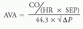
b. These variables are then used to determine valve area according to the following equation:

where CO = cardiac output (mL/min), HR = heart rate, SEP and DFP = systolic ejection period and diastolic filling period, respectively, C = constant, and ΔP = mean pressure gradient (mm Hg)
c. Gorlin validated this formula by comparing calculated values with measured mitral valve area (MVA) values in 11 patients (6 at autopsy and 5 during surgery). In this study, he noted a good correlation (within 0.2 cm2) between the calculated and measured valve areas.
d. Using these data, an empiric constant of 0.7 was derived for calculation of mitral valve area. Once left ventricular end-diastolic pressure (LVEDP) could be routinely measured, this value was adjusted to 0.85. The empiric constant has not been determined for aortic stenosis and an assumed value of 1 has been assigned. For patients with pulmonic and tricuspid stenosis, valve area is not routinely used, and mean pressure gradients are the predominant mechanism used to determine severity.
e. Using the Gorlin formula, MVA and aortic valve area (AVA) can be calculated as:

f. Examples:
i. Mitral stenosis: Assume a calculated Fick CO of 4.0 L/min, HR of 100 bpm, DFP 0.40 sec/beat, and ΔP of 25 mm Hg

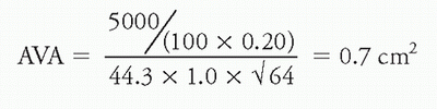
ii. Aortic stenosis: Assume a calculated Fick CO of 5 L/min, HR of 100 bpm, SEP 0.20 sec/beat, and ΔP of 64 mm Hg
2. Hakki equation
a. In an effort to simplify the process of invasive valve area calculation, Hakki et al. studied 100 consecutive patients (60 with aortic stenosis and 40 with mitral stenosis) who underwent combined left and right heart catheterization with calculation of valve area using the Gorlin equation. They observed that at normal HR, the product of HR, SEP or DFP, the constant, and 44.3 closely approximates 1,000 over a wide range of valve areas. With this in mind, they simplified the equation as follows:

where CO = cardiac output (L/min) and P = pressure gradient (mm Hg)
Using this equation, they noted a positive correlation between valve area calculations derived using the Gorlin and Hakki equations for patients with both aortic stenosis (r = 0.96) and mitral stenosis (r = 0.94).
b. In patients with aortic stenosis, the correlation was positive whether mean gradient or peak-to-peak gradient was used.
c. Care must be used when using this formula in patients with tachycardia, as the relative time spent in systole and diastole may change sufficiently at high HRs to render the basic assumptions used to derive this formula invalid.
d. Examples:
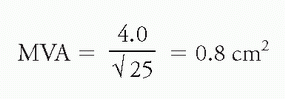
i. Mitral stenosis: Using the above values of CO = 4.0 L/min and ΔP of 25 mm Hg
ii. Aortic stenosis: Using the above values of CO = 5.0 L/min and ΔP of 64 mm Hg

B. Pressure gradients
As the cardiac valve becomes progressively narrower and resistance to flow consequently rises, higher pressure gradients are required in order to maintain adequate tissue perfusion. Although echocardiography has become the standard for determining these values in clinical practice, there are still scenarios where these calculations must be done in the cardiac catheterization laboratory. In these select cases, pressure gradients are directly measured rather than being indirectly obtained noninvasively using the simplified Bernoulli or continuity equation. If done with close attention being paid to best practice standards, such as the use of dual-lumen pigtail catheters with simultaneous LV to aortic pressure measurements for aortic stenosis, these measurements should be more accurate than the gradients obtained noninvasively. Failure to strictly adhere to these standards may result in inaccurate data acquisition and thereby clinical assessment.
1. Aortic stenosis
a. The LV-aortic gradient may be reported as:
i. Peak-to-peak gradient: refers to the difference between the peak aortic measurement and the peak LV measurement. Given that they are not temporally related, this measurement does not carry any physiologic significance, though it is often used to approximate mean gradient.
ii. Peak instantaneous gradient: represents the peak gradient that exists between the LV and aorta at any given point in time during the period of systolic ejection.
iii. Mean gradient: determined by integrating the area under the curve of the simultaneous LV-aortic pressure waveform. This measurement is the most reliable way for expressing the pressure gradient and the form used in calculating valve area via the Gorlin equation.
b. Technique:
i. Simultaneous LV-peripheral artery tracing: limited by both temporal delay and peripheral amplification of pulse waveform.
(a) Folland et al. directly compared simultaneous LV-aortic with LV-femoral arterial tracings and observed that in tracings that did not adjust for temporal delay, gradient was overestimated by a mean of 9 mm Hg, whereas the adjusted tracings underestimated gradient by a mean of 10 mm Hg.
ii. Simultaneous LV-aortic tracing via transseptal catheterization: Method of choice with mechanical aortic valves, in some cases when precise measurements of LV outflow tract (LVOT) gradients are needed (i.e., in patients with HOCM), or when the left ventricle is unable to be accessed via a retrograde approach.
(a) Limited use given invasiveness and consequent potential for complications.
iii. Simultaneous LV-aortic tracing via retrograde LV catheterization: This is the most common and preferred method. It can be done using a dual-lumen pigtail catheter or a single-lumen pigtail catheter in the aorta in combination with either a high-fidelity pressure wire or additional single-lumen pigtail catheter in the left ventricle.
2. Mitral stenosis
a. The mean gradient across the mitral valve may be determined either through direct left atrial (LA) cannulation via a transseptal puncture or using pulmonary capillary wedge pressure (PCWP) as a correlate for LA pressure.
i. Schoenfeld et al. studied 12 patients with prosthetic mitral stenosis and determined that the use of PCWP in this population consistently led to the overestimation of the mean gradient (13.2 mm Hg vs. 6.7 mm Hg) and consequent underestimation of MVA (mean 1.29 cm2 vs. 1.89 cm2). They postulated that this may have been due to (1) phasic delay in the PCWP V wave resulting in a higher mean diastolic pressure relative to the pressure obtained via use of direct LA pressure and/or (2) the recording of a dampened pulmonary artery pressure rather than a true PCWP tracing in patients with pulmonary hypertension.
IV. ANGIOGRAPHIC ASSESSMENT OF AORTIC AND MITRAL REGURGITATION
Although most commonly done through the use of Doppler echocardiography, there are certain scenarios when the use of angiography is needed to assess the degree of aortic or mitral regurgitation. The angiographic assessment of valvular regurgitation using the Sellers criteria for both the aortic and mitral valve is as follows:
A. Sellers criteria
1. 1+: Faint opacification of proximal chamber which clears with each beat
2. 2+: Mild opacification of proximal chamber which clears within a few beats
3. 3+: Moderate opacification of entire proximal chamber of equal intensity to the distal chamber
4. 4+: Intense opacification of proximal chamber to a greater degree than the distal chamber
V. AORTIC REGURGITATION INDEX
Given the correlation of increasing degrees of aortic regurgitation (AR) with post-transcatheter aortic valve replacement (TAVR) mortality, precise assessment of AR is crucial as a routine part of intraoperative care in this patient population. This remains difficult despite the routine use of invasive hemodynamics, aortography, as well as transesophageal echocardiography (TEE). Although not yet widely used in clinical practice, the AR index and time-integrated (TIAR) index were developed to help improve the accuracy by which postimplantation AR is measured.
A. AR index: Requires simultaneous determination of systolic blood pressure (SBP), diastolic blood pressure (DBP), as well as LVEDP, which are related as follows:

1. The complementary value of the AR index was prospectively assessed in 146 high-risk patients (mean Society of Thoracic Surgeons score = 9.8 ± 7.3%) who underwent implantation of a Medtronic CoreValve prosthesis. In this study, the AR index incrementally decreased with worsening AR and independently predicted 1-year mortality in patients with an AR index <25.
B. TIAR index: Attempts to improve the accuracy of the above assessment by integrating the representative pressures throughout their corresponding time in the cardiac cycle. It requires precise calculation of the LV-aorta (Ao) diastolic pressure time integral (DPTI) and LV systolic pressure time integral (SPTI).
1. LV-Ao DPTI: Represented by the integrated area between the central aortic and LV pressure waveforms during diastole.
2. LV SPTI: Calculated by integrating the area under the LV pressure waveform during systole.
3. These measurements can then be related to determine the TIAR index as follows:

4. In a study of 64 patients with severe aortic stenosis who underwent implantation of a Sapien valve, a TIAR index <80 predicted the presence of more than mild aortic insufficiency (AI) with a sensitivity of 86% and specificity of 83%. Furthermore, using receiver operating characteristic curve assessment, the TIAR index was associated with improved diagnostic accuracy compared to the AR index.
VI. FLUOROSCOPIC ASSESSMENT OF MECHANICAL VALVES
Occasionally, when either the presence of significant artifact limits the visualization of mechanical valves or falsely elevated noninvasive gradients are suspected due to pressure recovery, the use of fluoroscopic methods can be employed. This involves meticulously imaging the valve in a projection perpendicular to the plane of opening and closing of the prosthesis. Using these images, opening and closing angles can then be calculated and compared with standard values to determine whether or not significant obstruction is present (Fig. 22.1).
VII. REGURGITANT VOLUME AND REGURGITANT FRACTION
This concept was borne out of the desire to have a mechanism for quantitatively assessing valvular regurgitation in the cardiac catheterization laboratory. First described in 1963 by Sandler et al., it relies on the determination of the total LV stroke volume (TSV) as well as the effective forward stroke volume (FSV). Although not widely used, it will be briefly discussed here.
A. TSV: Defined as the difference between end-diastolic and end-systolic volumes as determined by left ventriculography.
B. FSV: Calculated by dividing CO (as determined by either Fick or thermodilution techniques, which measures effective forward flow) by HR.
C. These variables are then related according to the following equation to calculate regurgitant volume (RV):
RV = TSV – FSV
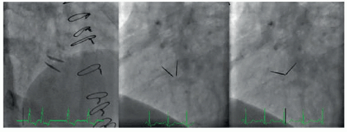 FIGURE 22.1 Fluoroscopic assessment of mechanical valves: In the left panel, it is evident that the image is obtained at an oblique angle, which would result in an inaccurate assessment of valve opening and closing. The center and right panels demonstrate proper orientation for measuring opening and closing angles in a separate patient with a mechanical aortic valve. The opening and closing angles represent the angle formed between the two leaflets in systole and diastole, respectively. These measurements can be compared to standard values in order to determine whether or not restriction is present. |
D. Using this information, regurgitant fraction (RF) can then be determined:
RF = (TSV – FSV)/TSV
E. Using this equation, mild = <20%, moderate = 21% to 40%, moderately severe = 41% to 60%, and severe = >60%.
F. Limitations:
1. Can be time-consuming and requires the use of highly sophisticated computerized software for calculating ventricular volumes.
2. The operator must ensure that representative volumes are obtained, as they may differ during each beat in the cardiac cycle. Of note, accurate volumes cannot be obtained in scenarios with variable R-R intervals, such as atrial fibrillation or frequent ectopic beats.
3. Error can also be introduced through inherent limitations involved in standard methods used to calculate CO.
4. The degree of valvular regurgitation is dependent on loading conditions of the LV, and as such, the operator must ensure that these remain consistent throughout the course of the procedure when measurements are being obtained.
VIII. CASE-BASED EXAMPLES
The remainder of the chapter will focus on case-based scenarios aimed at illustrating the clinical utility of the above techniques using a variety of hemodynamic loading conditions and provocative measures relevant to clinical practice. In addition to the above discussion, reference to Chapters 20 and 23 is encouraged to complement the information presented in the cases.
A. Aortic valve
Case 1: Normal flow with high gradient. A 68-year-old woman presented for further evaluation of worsening dyspnea on exertion. Her medical history is notable for hypertension, hyperlipidemia, pulmonary hypertension, moderately severe tricuspid regurgitation, heart failure with preserved ejection fraction (EF), and moderate aortic stenosis. She underwent a transthoracic echocardiogram, which demonstrated EF 65% with right ventricular systolic pressure 100 mm Hg, 3+ tricuspid regurgitation, and moderately severe aortic stenosis with mean gradient 33 mm Hg and AVA 1.0 cm2.
In order to further investigate the etiology of her symptoms, the patient was taken to the cardiac catheterization laboratory. Coronary angiography did not demonstrate any obstructive coronary artery disease (CAD). Right heart catheterization and simultaneous LV aortic pressure measurements were obtained using a dual-lumen pigtail catheter with the following results as shown in Figure 22.2.
Stay updated, free articles. Join our Telegram channel

Full access? Get Clinical Tree


