Blood Flow Measurements
Håkan arheden
Freddy Ståhlberg
BACKGROUND
Blood flow is a central physiologic parameter that can be measured, using magnetic resonance (MR) velocity techniques with high accuracy and precision, noninvasively, without ionizing radiation, in any part of the body and at any angle. Under normal physiologic conditions, blood flows with minimal resistance in conducting vessels. Disturbances to normal physiology, such as decreased pumping energy in heart failure, regurgitation in valve disease, increased resistance in stenosis, or rerouting of blood in shunting, can thus be quantified.
HISTORICAL OVERVIEW OF FLOW MEASUREMENTS WITH MAGNETIC RESONANCE IMAGING
Shortly after the first essential discoveries regarding the nuclear magnetic resonance (NMR) phenomenon (1,2), the effect of motion on the NMR signal was described, and the possible use of NMR for motion detection was investigated. Among the pioneers in this field were Suryan (3), who demonstrated a signalenhancing inflow effect from water flowing through an NMR probe; Bowman and Kudravcev (4), who proposed a method for the construction of an NMR blood flowmeter where this phenomenon was used; Singer (5), who proposed a motion-induced signal enhancement effect for measurements of blood flow; and Hahn (6), who developed a method for the detection of the motion of seawater using phase dispersion effects. In 1960, Grover and Singer (7) proposed a spin-echo-based method for the measurement of in vivo blood velocity distributions, while NMR flowmeters for the measurement of flow in the extremities using magnetic tagging of protons were developed by Battocletti et al. (8). Wash-out effects, creating an apparent T2 shorter than that for stationary spins were also used early for velocity measurements (9).
After the revolutionary introduction of NMR as an imaging modality (10), a large number of potential methods for the in vivo visualization and quantification of blood flow using magnetic resonance imaging (MRI) emerged. Flow effects were theoretically, as well as experimentally examined, and flow measurement methods with varying degrees of complexity were presented, ranging from straightforward methods, using standard sequences for the visualization of flow-induced signal voids, to quantitative methods requiring specially designed pulse sequences. Among the first to explore the field were Herfkens et al. (11), who stated that the information in a conventional MR image was flow dependent; Grant and Back (12), who showed wash-out effects in tubes; and Crooks et al. (13), who published a signalversus-velocity curve obtained with a spin-echo sequence. The possibility of using MRI for studies of obstructions in vessels was pointed out by, among others, Kaufman et al. (14) while Singer and Crooks (15), as well as Wehrli et al. (16), proposed quantitative methods for velocity measurements in vessels, based on wash-in/wash-out effects. Magnetic tagging methods, often known as bolus tracking or time-of-flight methods, were earlier proposed for use in MRI by Shimizu et al. (17). With respect to flow-induced phase effects on motion, the attenuation in modulus images as a result of phase spread or loss of phase coherence, within the voxel, was investigated by Waluch and Bradley (18), and the so-called even-echo rephasing effect was pointed out. Development along another line more directly took advantage of the phase-altering properties of motion. Here, the
theoretic framework was made by Moran (19), who proposed a method for the creation of velocity images by the addition of flow-sensitive or flow-encoding gradients to a standard pulse sequence. Several quantification methods using this basic idea were rapidly suggested (20,21) and led to clinical application.
theoretic framework was made by Moran (19), who proposed a method for the creation of velocity images by the addition of flow-sensitive or flow-encoding gradients to a standard pulse sequence. Several quantification methods using this basic idea were rapidly suggested (20,21) and led to clinical application.
As a result of the work outlined above, quantitative flow measurement sequences and evaluation tools have become available on standard MRI scanners, providing the possibility not only to measure velocity and flow, but also to evaluate important physiologic parameters, such as wall shear stress (WSS) and compliance. Furthermore, increased knowledge concerning flow effects in MR imaging has led to improved image quality in standard imaging because flowinduced image artifacts have been effectively reduced by the use of techniques such as flow refocusing, respiratory gating, retrospective/prospective ECG triggering, and presaturation.
Flow Measurement Techniques
In general, MR signal acquisition and image reconstruction mathematically requires so-called complex or vectorial treatment. After Fourier transformation in two dimensions of the spatially encoded signal, the reconstructed volume element (voxel) magnetization Mxy is obtained as a vector in the transverse or (x, y) plane. Mxy can be decomposed into real and imaginary parts according to Figure 5.1. MR images are normally displayed in absolute (modulus) mode, that is, the picture element (pixel) intensity is proportional to the length of the vector. This vector length is dependent on the object parameters (e.g., proton density, relaxation, flow, diffusion) as well as on acquisition parameters (echo time [TE], repetition time [TR], inversion time [TI], and so forth) and may hence be used for flow estimation.
Also possible is to reconstruct images where the intensity is proportional to the real or imaginary part of the vector or simply to the phase angle φbetween Mxy and the real axis. The latter type of image is referred to as a phase image and can, in principle, be reconstructed after acquisition of all types of pulse sequences. The phase angle is ideally independent of relaxation parameters and is zero in the absence of macroscopic motion. Presence of such motion will give rise to a flow-dependent phase angle, but caution should be taken regarding confounding phase effects introduced by, for example, nonlinear gradients, eddy currents, and concomitant gradients.
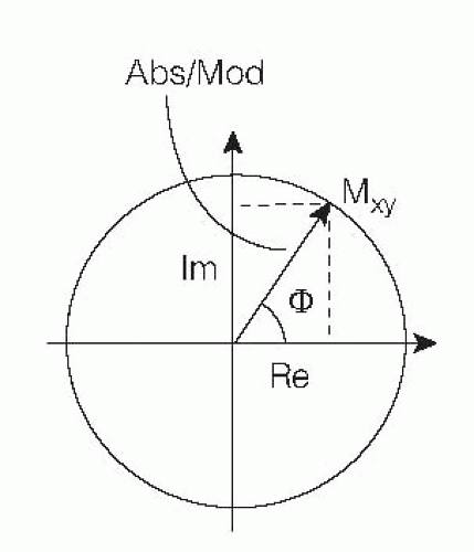 Figure 5.1. Illustration of different types of information in an MR image: The modulus or absolute value is the length of the signal vector, which creates a phase angle φ with the real axis. Components (Re) and (Im) are the projections of the modulus vector on the real and imaginary axis, respectively. |
On the basis of the type of image representation that is used, MRI flow measurement techniques are often divided into modulus-based and phase-sensitive techniques, respectively.
MODULUS-BASED TECHNIQUES
Slice-selective pulse sequences using two or more spatially selective RF pulses prior to the sampling of the echo are sensitive to the transport of spins into and out of the excited slice. If the flow has components perpendicular to the imaging slice, the signal will decrease owing to the outflow of spins during the time between RF pulses (wash-out). On the other hand, for sequences that require repetition, the inflow of nonsaturated spins during the TR will increase the magnetization compared with the static, saturated spins and thus give an increase in signal (wash-in). In a conventional spin-echo sequence, these competing mechanisms make the modulus signal behavior versus velocity biphasic and, possibly, difficult to interpret, although, with a rough knowledge of the velocities involved, the experimental parameters could be adjusted so that one mechanism is dominant. If, however, only one RF pulse is used prior to the sampling of the echo, as in basic gradient-echo sequences, the signal decrease due to wash-out will not occur, and wash-in effects may give prominent increase of vessel signal. For repeated sequences including multiple RF pulses—such as inversion recovery, fast spin-echo, and fast inversion recovery, as well as in multislice imaging— a complicated relation between velocity and signal is to be expected.
Wash-out and wash-in effects are predominantly used for qualitative evaluation of flow phenomena, and several clinically useful techniques have been proposed for this purpose. In cardiac applications, “black blood imaging” based on combined effects of wash-out phenomena and spin dephasing is used to visualize vessel walls in triggered multislice spin-echo imaging, whereas the inflow effect in gradientecho imaging forms the contrast basis in time-of-flight MR angiography, as well as in rapid cine imaging of the heart.
It has been shown that quantifying flow from transport effects reflected in modulus images is possible, if suitable models describing the signal-versus-velocity behavior are applied (16,22,23 and 24). However, signal-versus-velocity relations obtained using modulus images are generally nonlinear and influenced by relaxation times, which are difficult to determine accurately in vivo (25), and presently such methods are less frequently used than the phase-sensitive techniques described in more detail below. An alternative modulus-based method uses the so-called bolus tracking (17). Here, a bolus is first labeled or tagged with an RF pulse at a specific position and then observed downstream using a second RF pulse. Bolus tracking, which can be performed as a through-plane as well as an in-plane flow measurement method, is rapid and does not use relaxation time information, although methodologic drawbacks are, for example, that a minimum velocity is required, that the obtained information is generally not two-dimensional (2D) and that the method is best suited for nonpulsating flow. In this context, it should
be mentioned that several myocardial tagging techniques have emerged during the last years, as recently reviewed by Ibrahim (26). Based on early work by Zerhouni et al. (27) and Axel and Dougherty (28), techniques such as HARP (29), DENSE (30), and SENC (31) have shown the possibility for qualitative as well as quantitative evaluation of cardiac tissue motion, including determination of derived parameters such as strain.
be mentioned that several myocardial tagging techniques have emerged during the last years, as recently reviewed by Ibrahim (26). Based on early work by Zerhouni et al. (27) and Axel and Dougherty (28), techniques such as HARP (29), DENSE (30), and SENC (31) have shown the possibility for qualitative as well as quantitative evaluation of cardiac tissue motion, including determination of derived parameters such as strain.
PHASE-SENSITIVE TECHNIQUES
Background
As mentioned earlier, reconstruction of images is possible, where the intensity is proportional to the phase angle that the Mxy vector describes with the real axis. In MRI, the phase angle is used in the spatial-encoding procedure. After the Fourier decoding, ideally the phase information has been translated into position information, and no phase information remains. However, objects that move in a varying magnetic field (e.g., a pulsed gradient field) change their precession frequency and therefore obtain an offset phase angle not removed by the decoding procedure (19). The exact phase behavior for different types of gradients and motion patterns can be calculated, and a very simple linear relationship between constant velocity (so-called first-order motion) and phase angle is predicted by theory as well as confirmed in experiments. This relationship forms the basis for most of the clinically used flow measurement techniques in MRI. In its 2D form, the method is known by many names, for example, velocity mapping, phase mapping, or phase contrast MR (PC-MRI).
Theory
The Larmor equation states that the precession frequency f of a proton is proportional to the external magnetic field B, where the proportionality constant for protons in the hydrogen nuclei of water is 42.6 MHz/T. Since accumulated phase (φ) is proportional to the time integral of frequency, a proton will accumulate a phase shift proportional to the time integral of the magnitude of the magnetic field in each position.
In the presence of a linear magnetic field gradient along a direction x, the magnetic field at a position x can be described as B(x) = B0 + Gx(t) × x, where B0 is the main magnetic field (T) and Gx(t) is the time-dependent gradient (T/m) along the direction x (m). Hence, the additional phase shift introduced by the gradient can be calculated as
Consequently, application of a gradient will result in an additional phase shift according to the location along this gradient. Now consider application of two consecutive gradients with same duration and magnitude but with opposite sign (Fig. 5.2).
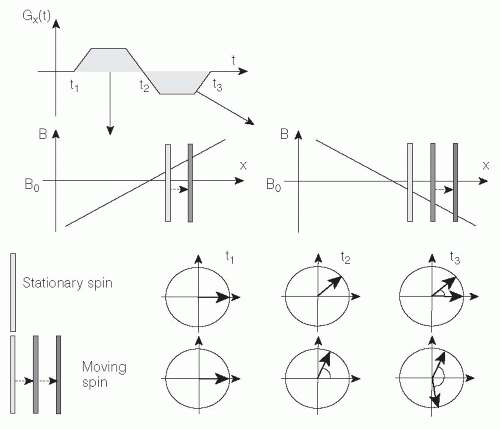 Figure 5.2. Application of two consecutive magnetic field gradients with same duration and magnitude but with opposite sign. When the first gradient is applied, all stationary protons will accumulate a phase shift determined by their location in the magnetic gradient field. Immediately after the first gradient, the second magnetic gradient is applied, and all of the stationary protons lose their accumulated phase shift and obtain a net phase shift of zero. A proton moving along the direction of the magnetic field gradients during their execution will experience unequal positive and negative magnetic gradients and, consequently, accumulate a net phase shift φ. |
When the first gradient is applied, all stationary protons will accumulate a phase shift determined by their location x according to Eq. 1. Immediately after the first gradient, the second gradient is applied and, again according to Eq. 1, all the stationary protons lose their accumulated phase shift and obtain a net phase shift of zero. This procedure is known as refocusing and is used in MRI to prevent gradient-induced signal dephasing along the slice-encoding and the frequencyencoding gradient directions. However, a proton moving along the magnetic field gradients during their execution will experience unequal positive and negative magnetic gradients and, consequently, accumulate a net phase shift φ. In the case of constant velocity v along x, the position of each proton can be written x(t) = v × t, and an additional velocitydependent phase shift φv is obtained from Eq. 2:
where the phase shift is proportional to the velocity along the magnetic gradient. Consequently, the phase image can
be regarded as a velocity map, where the phase shift in each voxel is proportional to velocity with a proportionality constant depending on the time course of the applied gradient in the investigated direction. Theoretically, the phase shift in voxels with stationary tissue should be zero, but additional phase shifts may be caused by many factors other than motion—for example, main magnetic field inhomogeneities, eddy currents, concomitant gradient effects, and local magnetic field gradients induced by magnetic susceptibility variations—but also by specific acquisition strategies, such as asymmetric echo sampling. These problems may be partly overcome by creating an additional phase image using a different set of gradient amplitudes which, in turn, gives a different velocity sensitivity or often no velocity sensitivity at all but with similar nonmotion-related phase shift behavior. Subtraction of these two phase images results in a velocity map, ideally showing φ = 0 for stationary voxels.
be regarded as a velocity map, where the phase shift in each voxel is proportional to velocity with a proportionality constant depending on the time course of the applied gradient in the investigated direction. Theoretically, the phase shift in voxels with stationary tissue should be zero, but additional phase shifts may be caused by many factors other than motion—for example, main magnetic field inhomogeneities, eddy currents, concomitant gradient effects, and local magnetic field gradients induced by magnetic susceptibility variations—but also by specific acquisition strategies, such as asymmetric echo sampling. These problems may be partly overcome by creating an additional phase image using a different set of gradient amplitudes which, in turn, gives a different velocity sensitivity or often no velocity sensitivity at all but with similar nonmotion-related phase shift behavior. Subtraction of these two phase images results in a velocity map, ideally showing φ = 0 for stationary voxels.
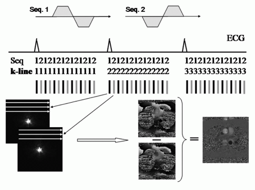 Figure 5.3. Prospectively, ECG-triggered velocity mapping with interleaving of two differently velocity-encoded sequences 1 and 2. After collection of a sufficient number of k-space lines for each sequence, pairs of raw data images are obtained for a number of time frames (cardiac phases) in the cardiac cycle. After Fourier transform, the resulting phase image pairs are subtracted to give the final phase map. Note that if synchronization is performed on every heart beat, k-space sampling is stopped prior to the end of the cardiac cycle because the R-R interval can be expected to vary in vivo, and hence end-diastolic phase maps cannot be obtained. |
Basic Sequences and Strategies for PC-MRI
Magnetic field gradients are present in all types of pulse sequences, and standard sequences usually exhibit some flow-dependent phase behavior unless this is specifically prevented by using motion-compensated gradient patterns. However, if flow is to be carefully quantified, additional gradients are applied to maximize the sensitivity for a particular velocity range since the velocity-to-noise ratio (VNR) in a phase map scales with the selected motion sensitivity as well as with the signal-to-noise ratio (SNR) in the corresponding modulus image (32).
Phase-sensitive flow MRI (henceforth denoted PC-MRI) is in its simplest form performed in single-slice mode, using two interleaved gradient-echo sequences with different flow sensitivity in one spatial direction (21,33), either through the imaging plane or in the imaging plane (2D PC-MRI). If flow is determined in the through-plane direction, either the slice-selective gradient can be redesigned to create sufficient velocity sensitivity or a bipolar gradient can be added in the slice-selective direction, although at the cost of prolonged TE. For in-plane measurements, either the frequency-encoding or the phase-encoding direction is used in a similar way for velocity sensitization. Subsequent complex voxelwise subtraction of the two phase images (34,35) will result in a net phase image where the phase shift is ideally determined only by motion, as shown in Figure 5.3.
An important prerequisite for PC-MRI of pulsatile motion is synchronization of the sequence execution to the time course of the flow pattern regulated by the cardiac cycle. Two strategies are commonly used for this purpose: Prospective ECG triggering and retrospective gating (36,37). In ECG-triggered PC-MRI, sampling of each phaseencoding line is triggered by the R-wave in the ECG (Fig. 5.3). The total number of image frames that can be obtained within an R-R interval depends upon the minimum sequence TR and the heart rate of the patient. Typical values for adults are 30 to 40 frames, but the number of frames will, as a rule, be lower in children as a result of a higher heart rate in children than in adults. ECG triggering involves drawbacks related to an almost certain change of the patient’s heart rate during the examination. Hence, it is difficult to obtain an image exactly at end-diastole during which atrial contraction occurs, unless the experiment is performed over two cardiac cycles. Furthermore, additional longitudinal relaxation in the delay time previous to each trigger pulse may lead to increased signal intensity and ghost artifacts in the first frames. These drawbacks can be overcome by using retrospective gating, where the MR signal is acquired continuously, asynchronously with the ECG. By postprocessing, the MR information is sorted and interpolated to fixed times in the cardiac cycle before reconstruction of the image frames. Although potential disadvantages in retrospective gating include signal manipulation, such as filtering and interpolation have been reported (38), Ley et al. (39) in a comparative study between ECG-gating methods concluded that retrospective ECG-gated free-breathing measurements allow for the most precise assessment of the bronchosystemic blood flow.
If the studied vessel also moves periodically in space because of respiratory motion, the basic strategy described above may not be sufficient. A method to overcome motion artifacts induced by respiration in PC-MRI is to use the
so-called segmented k-space technique, where the entire data acquisition can be made within a breath-hold by the sampling of several phase-encoding lines within a limited time window during each heart cycle (40,41). Although early studies have pointed out that the long acquisition windows introduced by the segmentation technique may cause unacceptable blurring in vessels moving rapidly with the cardiac rhythm (42,43), the use of techniques such as view-sharing (44) or shared velocity encoding (VENC) (45) can improve the temporal resolution, the latter technique also enabling real-time imaging.
so-called segmented k-space technique, where the entire data acquisition can be made within a breath-hold by the sampling of several phase-encoding lines within a limited time window during each heart cycle (40,41). Although early studies have pointed out that the long acquisition windows introduced by the segmentation technique may cause unacceptable blurring in vessels moving rapidly with the cardiac rhythm (42,43), the use of techniques such as view-sharing (44) or shared velocity encoding (VENC) (45) can improve the temporal resolution, the latter technique also enabling real-time imaging.
Furthermore, since breath-holding puts demands on the patient’s physical ability and has been shown to be inadequate for different subpopulations (46), several methods for combined synchronization to cardiac and respiratory motion during free breathing have been proposed. One example is the use of so-called navigators, a technique where a small excitation pulse is positioned, for example, over the diaphragm for monitoring of the patient’s breathing so that signal sampling is made only during end-expiration (47,48 and 49).
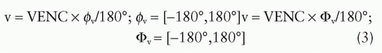
The resulting velocity-induced phase shift in the subtracted images can (without additional phase unwrapping) only be unambiguously determined in the phase angle interval (-180 degrees, +180 degrees). The velocity corresponding to a phase angle of 180 degrees is known as the VENC. The VENC can be calculated for a specific velocity-sensitive sequence pair, using Eq. 2. Using the VENC concept, velocity is obtained from measured phase angle by:
Basic parameters that can be determined from each time point in a velocity map with an adequately designed through-plane experiment are:
The (average) linear velocity in each voxel (cm/s): This basic parameter is obtained with direct use of Eq. 3. Mean velocity within a region of interest (ROI) is obtained by averaging linear velocities in each voxel within the ROI.
The cross-sectional flow area (cm2): An accurate way to obtain this parameter in stenotic vessels is to use the halfvalue of the maximum velocity (vmax/2) as threshold for pixels included in the orifice, giving a precision of over 90% for realistic orifice areas (50); see Section “Selection of Region of Interest.”
The volume flow (cm3/s): Found by multiplying the entire flow area with the mean velocity within it (Fig. 5.4).
Parameters such as net flow and stroke volume during an average heart beat, can be subsequently derived from the flow-versus-time curve in Figure 5.4, provided that the sampling is made over the whole cardiac cycle.
Technical Extensions of PC-MRI
Although most frequently performed with spoiled gradientecho sequences, the PC-MRI has also been combined with the balanced steady-state free precession (SSFP) pulse sequence (51,52). Since the SNR in blood is higher in SSFP acquisitions compared to gradient-echo acquisitions, the combination of SSFP and PC-MRI is favorable in terms of reduced phase noise.
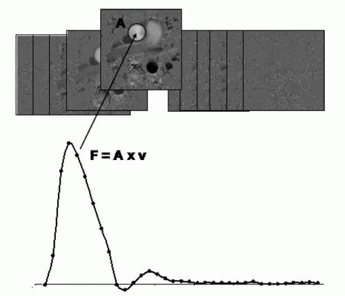 Figure 5.4. Calculation of a flow-versus-time curve from timeseparated phase maps. Volume flow F is obtained using the relation F = v × A for each phase map, where A is the area of the region of interest (ROI) encompassing the vessel and v is the average velocity measured in the ROI. |
PC-MRI can also be extended to all three spatial directions, although, for time-resolved measurements, at the cost of prolonged acquisition time or reduced temporal resolution, because in such a case at least four images (one reference image and three velocity-sensitized images in each geometrical direction) has to be obtained to create subtracted net phase images for each time point in the cardiac cycle. The dimensional extension has been referred to as, for example, time-resolved three-dimensional (3D), four-dimensional (4D), or even seven-dimensional (7D) flow imaging, the latter referring to three VENC dimensions, three spatial dimensions, and time resolution as one dimension. Initial suggestions for this extension emerged already in the 1990s (53,54), and thereafter proposals for methodologic development of the technique, here denoted 4D PC-MRI, as well as suggestions for potential clinical applications have been numerous (55), as also described in the following.
Several methods for reduction of the acquisition time in PC-MRI have been suggested. For example, strategies using reduction to one spatial dimension (56,57 and 58) give possibilities for either dynamic recording of flow in 1D projections or full so-called Fourier VENC within a reasonable acquisition time, and spiral readout techniques allow for real-time 2D PC-MRI (59). Echo-planar imaging methods for flow quantification using the PC-MRI strategy have been proposed for 2D PC-MRI as well as for 4D PC-MRI in vessels and structures with a reasonably large area (60,61 and 62).
Reduction of acquisition time in PC-MRI can also be achieved by combination with scan-time reduction strategies, such as k-t-BLAST and SENSE (63). Initial evaluations show that PC-MRI in combination with parallel imaging reconstruction can be accurately performed at reasonable reduction factors (64,65 and 66), while k-t-BLAST holds promise to reduce scan times in SSFP PC-MRI and Fourier VENC (67,68). Both techniques have been evaluated for 2D as well as for 4D PC-MRI (69,70).
Potential Error Sources
By now, the PC-MRI technique, and especially in its 2D form with VENC in the through-plane direction, has been thoroughly validated. For an overview of validation results, please see later Section “Validation.” Nevertheless, several sources of error might hamper the accuracy of a PC-MRI measurement, and such error sources are described in the next section.
ALIASING AND SLICE MISALIGNMENT. As stated previously, the net phase shift can only be unambiguously determined in the phase angle interval (-180 degrees, +180 degrees) and hence, velocities resulting in phase angles outside this interval will result in wrapped or aliased phase information. To avoid aliasing, a certain a priori knowledge of expected velocities in the investigated vessel is useful. If average flow (F) and vessel area (A) can be estimated, average velocity (v) is easily calculated by v = F/A, and assuming laminar flow in the vessel, the highest expected velocity is vmax = 2 × v. By setting VENC slightly higher than vmax, aliasing can be avoided. Methods to correct for aliasing (socalled unwrapping) have been proposed (72,73), but these techniques are rarely included in standard scanner software. In this context it should be noted that if VENC is increased to avoid aliasing, the velocity sensitivity is reduced and thereby also VNR. Accordingly, strategies for VENC adaption during execution of the PC-MRI sequence have been proposed (74,75).
Misalignment between the direction of flow and the direction of the motion-encoding magnetic gradients may also lead to erroneous MR velocity measurements. The phenomena can be avoided in through-plane PC-MRI by careful adjustment of the imaging plane so that it is aligned perpendicular to the flow direction. However, if the angle φ of misalignment is known, then the true velocity value vtrue can theoretically be calculated from the measured value vmea using vmea = vtrue × cos φ. In the absence of partial-volume errors, a misalignment of as much as 20 degrees will produce only a 6% error, whereas a more realistic misalignment of 5 degrees causes an error <1% (76). Volume flow measurements are ideally unaffected by misalignment because the measured cross-sectional area increases proportionally to the decrease in vmea; however, in practice partial-volume errors may result in overestimation of flow in the presence of misalignment (77).
SELECTION OF REGION OF INTEREST. A general, and perhaps slightly overseen, problem hampering accurate volume flow measurements, specifically in through-plane applications, is the selection of the position, size, and shape of the ROI that encompass the vessel. Ideally, average flow can be calculated by the product between average velocity and ROI area, that is, F = v × AROI, provided that the ROI area is chosen equal to or larger than the cross-sectional vessel area, while selection of an area smaller than AROI will lead to flow underestimation. For larger vessels at normal resolution and SNR level, selection of an ROI slightly larger than AROI will give accurate values of F (78).
A different type of problem becomes important, if the number of pixels per vessel diameter (Nd) is low, a situation occurring for imaging of smaller vessels and cavities or even for intermediate vessel sizes at low spatial resolution. In this case, partial-volume effects at the edges of the vessel may become significant (79). The partial-volume effects originate from within a voxel where stationary and flowing tissue is mixed, and the modulus signal is a vector summation between signals from these two compartments. The net phase angle will correctly relate to average voxel velocity, only if magnitude signal components reflect the concentration relation between the two compartments. Normally, flowing liquid has higher magnitude than stationary tissue in a through-plane investigation as a result of inflow effects, and the net phase angle may therefore overestimate velocity if an ROI is chosen so that all edge pixels are included. Errors may reach over 10% if Nd ≥ 5 (79). Several methods for reduction of the partial-volume effect have been suggested, for example, selection of an ROI slightly smaller than the entire visible flow area (53,77), empiric corrections based on phantom measurements (80), thresholding in combination with seed-growing (81), magnitude-based corrections (82), corrections based on complex difference (CD) techniques (35), automatic active contour models (83), and methods based on point-spread function shapes (84).
Furthermore, regardless of vessel size, great care must be taken that AROI does not encompass areas with signal at or close to the noise level (e.g., air spaces), because in such areas the phase value will be random unless the phase image is post-processed to give zero phase. Hence, the proper placement of the ROI may require inspection of modulus, as well as phase images (85,86).
BACKGROUND CORRECTION. As described earlier, several factors may contribute to the net phase information in an MR phase image. The subtraction routine in PC-MRI outlined previously is intended to cancel all phase effects not related to encoding of motion, but residual effects are unavoidable and may cause significant errors, for example, when flow over a whole cardiac cycle is calculated from a large number of time-resolved phase maps (87). Several reasons for nonzero phase background can be found.
First, the use of alternating magnetic gradient fields induces eddy currents in the conducting parts of the MR system (88). These eddy currents generate transient magnetic fields, which create phase offsets that vary linearly in space. Since different gradient patterns are used in the two sequences in a basic PC-MRI experiment, different phase effects can be expected, and a residual phase effect will appear in the subtracted image.
Second, when magnetic field gradients are applied for image formation and VENC, concomitant magnetic fields are created in accordance with Maxwell’s equations. These additional magnetic fields may create significant errors in velocity measurements (89) because, again, different gradient patterns are used in the two basic sequences, giving a net effect from concomitant gradients in the subtracted phase image. It should be noted that effects from concomitant
gradients scale quadratically with gradient amplitude and distance from the magnet isocenter but inversely with magnetic field strength. The largest effects can be anticipated in measurements performed at positions significantly displaced from the isocenter with a combination of strong magnetic field gradients and low main magnetic field strength (90).
gradients scale quadratically with gradient amplitude and distance from the magnet isocenter but inversely with magnetic field strength. The largest effects can be anticipated in measurements performed at positions significantly displaced from the isocenter with a combination of strong magnetic field gradients and low main magnetic field strength (90).
Third, nonlinearity in the applied magnetic field gradients can be caused by the finite size of the coils in the gradient system. In the images, gradient nonlinearities result in image distortion as a result of differences between the actual and expected magnetic field strengths. In the case of PC-MRI, nonlinear gradients will introduce differences between expected and actual VENC and, similar to the Maxwell effects, these errors become more prominent the more distant the investigated voxels are from the isocenter of the magnet.
Consequently, several methods for background phase corrections have been proposed. Removal of linear phase effects can be done by modeling linear functions based on the measured background in the stationary regions in the image (32,91). Correction is then achieved by subtracting the position-dependent modeled background phase from measured phases in the vessel. A simplified version of linear correction is to select two ROIs on opposite sides of and at equal distances from the vessel, and subtract the average background phase value from the vessel data (92). However, selection of adequate background ROIs may be difficult, especially in the thoracic region. Other more advanced methods include combined noise reduction and semiautomatized background correction (93), and correction methods for errors caused by nonlinear gradient fields (94,95).
In summary, although technical developments such as the use of self-shielded gradient coils and the use of builtin analytical corrections for concomitant gradients may reduce the phase offset problem substantially, in our opinion other development lines such as the use of increased gradient strengths, shorter magnets and gradient coils, and larger magnet bore sizes may act in the opposite direction. The effects of background phase should therefore certainly not be neglected in precise velocity and volume flow measurements using PC-MRI. In fact, background errors in modern MRI scanners appear to be highly variable in multicenter comparisons (96).
PHASE DISPERSION. In PC-MRI, each voxel may contain a spectrum of velocities as well as higher-order motion components, such as acceleration and jerk. This inhomogeneity of motion components will give rise to a distribution of phase shifts within the voxel (phase dispersion). The net flow-induced phase shift within a voxel is obtained from a vectorial summation of all of the elementary phase contributions, and, when this vectorial summation is made, several situations can occur that will affect the phase-versus-velocity linearity. For example, errors in velocity estimated from average voxel phase may occur, if modulus signal differs within the voxel because of different degrees of inflow enhancement (97). Furthermore, phase dispersion inevitably leads to loss of magnitude signal and increased uncertainty in the corresponding phase information. In extreme cases phase information cannot be unambiguously determined, and the linearity between velocity and measured phase is lost.
In PC-MRI of laminar flow the phase-velocity relation is, however, generally preserved. When the Reynolds number (which is related to the ratio between velocity and viscosity of the liquid) is increased, the flow profile changes and at very high Reynolds numbers, a flat velocity profile, although randomly fluctuating in time at every position, is obtained (turbulent flow). However, even with this time-dependent random motion, there is a well-defined average velocity profile in the vessel, and the instantaneous velocity at a point is given by this average velocity plus the fluctuating velocity at that instant. Transition from laminar to turbulent flow in straight, smooth-walled vessels is not associated with a decreased modulus signal in gradient-echo imaging (98), and the phase-velocity relation in PC-MRI is not affected, owing to that the so-called turbulent intensity (the ratio between fluctuating velocity and average velocity) in a turbulent flow field is relatively low in such cases (99).
Another situation may occur in a constriction, where so-called separated or complex flow is at hand. It has been shown that if a constriction is present, turbulence intensity values may drastically increase (99). Although several other explanation models, such as influence of higher-order motion, have been proposed (100), fluctuations of velocity in time as well as in space might be the most important reason for reduction in modulus signal and breakdown of phaseversus-velocity linearity after a constriction. Systematic investigations using flow phantoms have revealed that several factors in relation to the complex flow patterns influence the phase-versus-velocity linearity. Thus, for a given volume flow, the breakdown in linearity becomes more pronounced as the cross-sectional area of the constriction is reduced. Furthermore, for a certain constriction the phase-velocity relation is more likely to become nonlinear as the volume flow increased. Even though the phase-velocity relation is regained as the imaging plane for MR velocity mapping is moved downstream the constriction, disturbances may appear several centimeters distal to the tightest constrictions. Regardless of the correct explanation model for such findings, results from several groups show that a reduction of TE, or, more formally, VENC gradient duration, will reduce signal loss and regain unambiguous phase information (100,101,102 and 103). In this context, it should be mentioned that radically reduced TEs can be achieved with so-called UTE (ultrashort TE) sequences, which have recently been proposed for flow quantification in complex flow fields (104).
DISPLACEMENT. IN MR imaging of flow, time differences between phase and frequency encoding may lead to a displacement artifact that is manifested as a distortion of the vessel lumen (105) and which can be prominent for rapid flow moving obliquely relative to these gradients. Alternative names for this phenomenon are misregistration and oblique flow artifact.
Furthermore, when the moving spins are subjected to acceleration and other higher orders of motion, the obtained phase shift no longer depends solely on velocity, and Eq. 2 does not hold (106). The induced phase shift in the presence of higher orders of motion has been identified as a potentially confounding factor in velocity measurements (107), but it can be further analyzed theoretically by so-called Taylor expansion of the expression for the position x(t) of
a spin as a function of time. According to such analysis, the total phase shift in a bipolar experiment can be regarded as a velocity measurement free from the influence of higher-order motion but spatially misplaced in the reconstructed velocity image owing to differences in time between true VENC, occurring at the so-called moment center time or gravity center and spatial encoding (106,108,109).
a spin as a function of time. According to such analysis, the total phase shift in a bipolar experiment can be regarded as a velocity measurement free from the influence of higher-order motion but spatially misplaced in the reconstructed velocity image owing to differences in time between true VENC, occurring at the so-called moment center time or gravity center and spatial encoding (106,108,109).
Displacement errors can therefore be expected when measuring physiologic flows in the heart and great vessels with the phase-contrast technique. One way of reducing the oblique flow artifact is to reduce the time difference between phase and frequency encoding and, similarly, the displacement effects of higher-order motion components can be reduced by reduction of the time difference between the true VENC time and the time for spatial encoding (110).
CALCULATION OF DERIVED PARAMETERS. Apart from blood flow measurements, there are many examples where the acquired velocity data can be used for extended visualization of flow patterns (e.g., based on virtual particle behavior) as well as for calculation of different physiologic parameters derived from the velocity data. From PC-MRI data, visualization of flow can hence be made, for example, using velocity vector mapping, streamline visualization, pathline visualization, and volume tracking (111,112,113,114 and 115); the three latter techniques developed for 4D PC-MRI (Fig. 5.5).
Furthermore, several quantitative parameters of physiologic value can be derived as described below.
The transstenotic pressure gradient (in case of stenotic vessels), which gives information about the severity of constrictions in the vessels, can be estimated by inserting vmax (m/s) in the stenotic jet in the modified Bernoulli equation ΔP = 4 = vmax2 (116). However, the simplified Bernoulli equation is based on several assumptions, for example, that the velocity of blood is zero before the constriction. The measurement accuracy of this parameter can also be compromised by partialvolume effects and malpositioning of the imaging slice (50). In this context it should be mentioned that the magnitude of the signal from PC-MRI can be used to measure the standard deviation of the velocity distribution within a voxel, in turn giving possibilities to measure parameters related to turbulence, such as the turbulent kinetic energy (TKE) (117).
A proposed marker for localization of areas where formation of atherosclerosis will appear is the WSS (118). The calculation of the WSS τ is given by τ = µ × dv/dr, where the quotient dv/dr corresponds to the velocity gradient at the vessel wall and µ is the viscosity, which for the blood is 0.004 N s/m2. Several studies have shown the possibility of calculating the WSS in vessels using MRI velocity data (119,120), recently including 4D PC-MRI measurements also encompassing the oscillatory shear index (OSI) which describes the existence and magnitude of WSS changes over the cardiac cycle (121).
Another parameter of clinical interest which can be measured with 2D as well as 4D PC-MRI is the velocity of propagation of a pulse wave along a vessel, the pulse wave velocity (PWV) which relates to aortic stiffness (122). Furthermore, the elasticity of the greater blood vessels can be assessed by calculation of the vascular compliance. Compliance provides an estimate on the vessel conditions because low compliance is associated with a number of different cardiovascular diseases whereas large values correlate to overall fitness and youth. It has been shown feasible to calculate vascular compliance using time-resolved velocity data (123).
The contraction and relaxation of the pumping heart imply varying strains in different regions of the myocardial muscle. Quantification of strain and strain rate in the myocardium has been suggested as methods to identify ischemic areas in the heart, and velocity data in the myocardium can be used to calculate strain rate (124,125 and 126). In the case of velocity-mapping-based strain and strain-rate calculations, no tracking of fictive markers has to be performed because the measured velocities provide enough information for the calculation of this parameter.
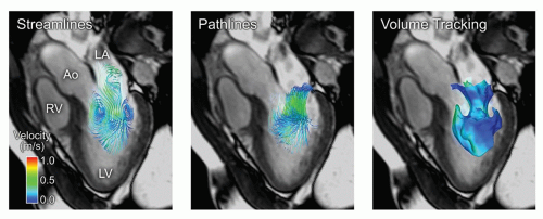 Figure 5.5. Comparison of three methods for visualization of blood flow in the human heart during rapid filling of the left ventricle. Blood flow was measured using 4D phase contrast magnetic resonance (4D PC-MR). Left: Streamlines are lines that are instantaneously tangent to the flow. Middle: Pathlines, released near the mitral annulus during rapid filling. Pathlines show the path of virtual particles released in the flow. Note that streamlines and pathlines differ in pulsatile flows such as the heart and great vessels. Right: Volume Tracking (114) of the blood flowing into the left ventricle. The blue surface separates the blood flowing from the left atrium into the left ventricle from the blood that was already in the ventricle. LV, left ventricle; LA, left atrium; Ao, aorta; RV, right ventricle. Color scale: velocity. |
In this context, it should be noted that with the evolution of PC-MRI, possibilities to compare measured PC-MRI data
with results from computed fluid dynamic (CFD) modeling in the cardiovascular system (127), and also to use PC-MRI data as input for improved CFD analysis on a patient-topatient basis has emerged, as shown for example by Wood et al. (128) and Torii et al. (129).
with results from computed fluid dynamic (CFD) modeling in the cardiovascular system (127), and also to use PC-MRI data as input for improved CFD analysis on a patient-topatient basis has emerged, as shown for example by Wood et al. (128) and Torii et al. (129).
Validation
In our opinion, flow velocity mapping sequences used for clinical or scientific purposes should be validated in-house before implementation. The reasons for this are twofold: First, the investigator should be familiar with the error sources described in the previous section and their effects in the investigator’s own equipment environment and second, hardware and software are continuously updated, and new flow velocity sequences are developed and delivered automatically with new software updates.
Validation of the specific flow sequence can be performed both in vitro using a flow phantom and in vivo where flow conditions can be assumed to be completely normal, as in healthy volunteers or in patients where flow velocities can be compared to Doppler ultrasound.
Lately, perhaps due to introduction of newer versions of hardware and software, some investigators have had reasons to believe that flow measurements may have become less robust (130,131). A multicenter, multivendor study using standard clinical flow sequences in standard measurement planes demonstrated significant phase offset errors when applied to a static gelatin phantom (132). These types of errors are individual to each individual scanner and can be accounted and corrected for in each scanner underscoring the need for in-house validation of flow sequences. Vendors and the scientific community are well aware of these challenges, work together to provide a solution, and should be able to provide advice on these matters.
VALIDATION IN VITRO
Volume flow and velocity have been validated in vitro using flow phantoms. In 1984, Bryant et al. (133) described a conventional spin-echo sequence with balanced gradient pulses on either side of the pi radiofrequency pulse and showed that the flow rate measured by MR agreed with the volume flow rate through a constant flow phantom. Several studies have confirmed high accuracy and precision of MR volume flow quantification in vitro, using phantoms with constant (92,134,135,136 and 137) or pulsatile flow (77,138,139,140,141


Stay updated, free articles. Join our Telegram channel
Full access? Get Clinical Tree
