Assessment of Perioperative Hemodynamics


Assessment of Perioperative Hemodynamics


Lee Wallace


While M-mode and two-dimensional (2-D) echocardiography can provide indirect evidence of hemodynamic abnormalities, 2-D echocardiography combined with Doppler echocardiography can be used to perform a quantitative hemodynamic assessment. Quantitative hemodynamic data that can be obtained with 2-D Doppler echocardiography are listed in Table 22.1.

The accuracy of many of these Doppler-derived measurements has been validated in the cardiac catheterization laboratory using transthoracic echocardiography (1,2,3,4). The principles on which these measurements are based hold as true for transesophageal echocardiography (TEE) as they do for transthoracic echocardiography. The accuracy of a hemodynamic assessment performed using either transthoracic echocardiography or TEE is dependent on the ability of a knowledgeable and skilled echocardiographer to acquire accurate data. The accuracy of the hemodynamic data acquired using either approach depends on the following: parallel alignment of the ultrasound beam with the blood flow of interest, minimal interference from adjacent blood flows, and for many calculations, an accurate determination of area or diameter.

Prior to the introduction of multiplane TEE probes, transthoracic echocardiography was considered a superior approach because it offered far more echocardiographic windows for interrogation of blood flow. The introduction of multiplane TEE probes has significantly increased the number of windows and angles from which blood flows may be interrogated. Furthermore, the introduction of high frequency transducers into multiplane TEE probes has aided in the accurate measurement of areas and diameters such that TEE may be superior to transthoracic echocardiography in many instances. Nevertheless, in order to avoid misdiagnosis, Doppler-derived measurements must be considered in the context of the quality of the acquired data as well as the overall hemodynamic status of the patient. This is especially true when using the transesophageal approach in the operating room setting. This chapter will focus on quantitative hemodynamic assessment using 2-D Doppler echocardiography. M-mode and 2-D echocardiographic signs of hemodynamic abnormalities, determination of diastolic function with Doppler, and estimation of cardiac-filling pressures based on diastolic parameters will be discussed in more detail in other chapters.


DOPPLER MEASUREMENTS OF STROKE VOLUME AND CARDIAC OUTPUT


Calculation of Stroke Volume

The flow rate of a fluid through a fixed orifice is directly proportional to the product of the cross-sectional area (CSA) of the orifice and the flow velocity of the fluid
within the orifice as given by the hydraulic orifice formula (Fig. 22.1):


TABLE 22.1. Hemodynamic Data Obtainable with 2-D Doppler Echocardiography


Volumetric measurements


Stroke volume


Cardiac output


Pulmonary-to-systemic flow ratio (Qp/Qs)


Regurgitant volume and fraction


Pressure gradients


Maximum gradient


Mean gradient


Valve area


Stenotic valve area


Regurgitant orifice area


Intracardiac and pulmonary artery pressures


Right ventricular systolic pressure


Pulmonary artery systolic pressure


Pulmonary artery mean pressure


Pulmonary artery diastolic pressure


Left atrial pressure


Left ventricular end-diastolic pressure


Ventricular dp/dt


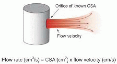
FIGURE 22.1. The hydraulic orifice formula. The volumetric flow rate through an orifice is equal to the product of the cross-sectional area of the orifice and the flow velocity of the fluid through the orifice. If flow velocity is constant, so is flow rate; however, if flow velocity varies, so will flow rate. CSA, cross-sectional area.

Flow rate (cm 3/s) = CSA (cm2) × Flow velocity (cm/s)

Because the cardiovascular system is pulsatile, blood flow velocity varies. Nevertheless, the instantaneous flow rate of blood going through an orifice or blood vessel of constant cross-sectional area is directly proportional to the product of the cross-sectional area (CSA) of the orifice or blood vessel and the instantaneous blood flow velocity.

The acceleration and deceleration of blood flow velocity during the ejection period (or filling period) provides a distinct Doppler profile for a given orifice. The summation of velocities over the entire flow period is correctly called the velocity-time integral (VTI), although it is also commonly referred to as the time-velocity integral (TVI). The VTI is equal to the area bounded by the Doppler flow velocity profile and the zero velocity baseline (Fig. 22.2). It is measured by tracing the Doppler velocity signal using the calculation package built in the ultrasound machine. The VTI can be conceptually thought of as the distance that blood travels with each beat of the heart and is thus also called the stroke distance.

Stroke volume (SV) can be calculated as the product of the cross-sectional area and VTI (Fig. 22.3):

SV (cm3) = CSA (cm2) × VTI (cm)

Stroke volume can be calculated at many different locations within the heart or great vessels by using the appropriate Doppler velocity signal to determine the VTI at the same location that 2-D imaging is used to determine cross-sectional area. Accordingly, the VTI is usually measured with pulse wave Doppler. However, continuous wave Doppler may be utilized to determine the aortic valve VTI in the absence of subvalvular or supravalvular aortic obstruction. In this case, the velocity signal obtained by continuous wave Doppler across the aortic valve should be the same as that obtained by pulse wave Doppler within the aortic valve.


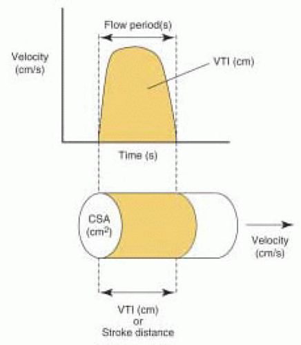
FIGURE 22.2. The Doppler velocity-time integral and stroke distance. As flow in the heart and great vessels is pulsatile, blood flow velocity varies during the period of ejection (or filling) as shown by the Doppler velocity curve. The area under the Doppler velocity curve (the velocity-time integral) is equivalent to the distance blood flow travels with one beat of the heart (stroke distance). VTI, velocity-time integral; CSA, cross-sectional area.

Most often the cross-sectional area of the “orifice” to be measured is assumed to be circular and thus can be calculated using the formula for the area of a circle (of radius r) after measuring the orifice diameter (D) in cm:

CSA (cm2) = II × r2 = II × (D/2)2 = 0.785 × D2

The Doppler method for determining stroke volume at a particular site is based on the following four assumptions, which are listed in Table 22.2. First, blood flow is assumed to be laminar and the spatial flow velocity profile is assumed to be flat, as is generally the case in the LVOT (Fig. 22.4). The narrow band of velocities and smooth spectral signal obtained with pulsed wave Doppler is evidence of laminar flow in the great vessels and across normal cardiac valves. A flat flow velocity profile can be demonstrated by showing uniform velocities while moving the pulsed wave Doppler sample volume from side to side within the flow of interest from two orthogonal views.


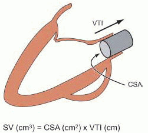
FIGURE 22.3. Doppler stroke volume calculation. The velocity-time integral of the Doppler velocity curve can be conceptualized as the length of a cylinder of blood (stroke distance) ejected through a cross-sectional area on one beat of the heart. Stroke volume is calculated as the product of cross-sectional area and the velocity-time integral. SV, stroke volume; CSA, cross-sectional area; VTI, velocity-time integral.

Second, cross-sectional area (i.e., diameter) and VTI measurements are assumed to be made at the same time and at the same anatomic location. Diameter is measured most accurately when the ultrasound beam is perpendicular to the blood-tissue interface, while VTI is measured most accurately when the ultrasound beam is parallel to blood flow. Thus, diameter measurements and Doppler velocity profiles are usually not recorded from the same imaging plane. Nevertheless, every effort should be made to perform these measurements at the same anatomic location and in close sequence in order to minimize error in the calculated stroke volume.


TABLE 22.2. Assumptions for Accurate Doppler Stroke Volume Calculations


1.


Blood flow is laminar with a spatially flat flow velocity profile.


2.


Measurements of the velocity-time integral and cross-sectional area (i.e., diameter) are made at the same time and at the same anatomic location.


3.


The velocity-time integral measurement represents the average velocity-time integral (several measurements should be averaged for a patient in normal sinus rhythm, whereas 8 to 10 should be averaged for a patient in atrial fibrillation).


4.


Cross-sectional area (i.e., diameter) measurement is accurate.


5.


The velocity-time integral is measured with the Doppler beam parallel to blood flow (i.e., θ = 0 in the Doppler equation) in order to avoid underestimation.


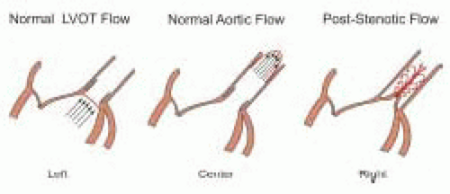
FIGURE 22.4. Common flow patterns. Left: Acceleration of blood within the left ventricular outflow tract leads to laminar flow with a flat velocity profile. Center: Friction along the wall of the ascending aorta leads to laminar flow with a parabolic flow profile. Right: Aortic stenosis results in a narrow, high velocity laminar jet originating from the stenotic orifice surrounded by turbulent flow.

Third, the VTI used in calculating stroke volume is assumed to represent the average VTI. Therefore, several measurements should be averaged for a patient in normal sinus rhythm, whereas between 8 and 10 measurements should be averaged for a patient in atrial fibrillation, in order to most accurately estimate the average VTI.

Fourth, determination of cross-sectional area is assumed to be accurate. Changes in cross-sectional area during the flow period, or deviations from an assumed geometry (usually circular) are inherent problems in Doppler stroke volume calculations. Accurate determination of 2-D measurements for calculation of cross-sectional area is essential. In the case of an assumed circular orifice, a small error in diameter measurement will result in a large error in the calculated cross-sectional area due to the quadratic relationship between the radius and area of a circle (i.e., CSA = II × r2). The use of high frequency multiplane TEE probes for measuring diameters (or areas) undoubtedly increases the reliability of these measurements when compared to the use of lower frequency monoplane or biplane TEE probes.

Fifth, the VTI is assumed to be recorded with the ultrasound beam parallel to the flow (i.e., the intercept angle θ = 0). In this case the velocities measured by Doppler are accurate based on a cosine θ = 1 in the Doppler equation (Fig. 22.5). However, as θ increases from 20° to 60°, the error in the calculated Doppler velocity increases from 6% to 50% (Fig. 22.6). Small adjustments in the TEE probe transducer position and the pulsed wave Doppler sample volume (or continuous wave Doppler beam) are necessary to obtain the highest velocity signal. Multiple imaging planes should be utilized when possible to ensure that the highest velocity signal is obtained. Use of the audio Doppler signal in addition to the visual Doppler display may aid the echocardiographer in optimal alignment of the ultrasound beam with the flow of interest. The highest velocity signal obtained (the loudest audio signal) will correlate with the most parallel alignment
of the Doppler beam with blood flow. While underestimation of velocities is always a potential source of error in Doppler stroke volume determination with TEE imaging, it is undoubtedly less of a concern with multiplane than with monoplane or biplane TEE imaging.


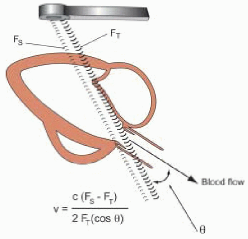
FIGURE 22.5. The Doppler equation. Blood flow velocity can be calculated based on the Doppler shift, which is the change in frequency between transmitted and backscattered ultrasound. v, blood flow velocity; c, the speed of sound in blood; FT, the frequency of transmitted ultrasound; FS, the frequency of backscattered ultrasound (the ultrasound reflected from moving red blood cells); θ, the angle between the blood flow and interrogating ultrasound beam.


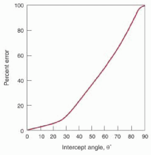
FIGURE 22.6. Velocity measurement error due to a nonparallel intercept angle. This graph shows the percentage error in the velocity calculation using the Doppler equation if the intercept angle between blood flow and the ultrasound beam is erroneously assumed to be zero. θ, the true angle between blood flow and the interrogating ultrasound beam.


Calculation of Cardiac Output

Cardiac output (CO) can be estimated with 2-D Doppler after determining a Doppler stroke volume and measuring heart rate (5). Cardiac output is calculated as the product of stroke volume and heart rate (HR). Cardiac index (CI) is calculated by dividing cardiac output by body surface area (BSA):

CO (l/min) = SV (cm3) × (1 liter / 1000 cm3) × HR (bpm) CI (l/min/m2) = CO (l/min) / BSA (m2)

Cardiac output measurements performed with TEE, usually measured at the LVOT or aortic valve in the absence of aortic regurgitation, have been shown to correlate well with measurements made by thermodilution (6,7,8,9,10,11). An accurate estimation of cardiac output depends on accurate determinations of the VTI and cross-sectional area. It is advisable to interrogate from multiple windows when possible. Accuracy is improved by assessing multiple Doppler flow profiles, typically 3-5 for a regular rhythm and 10 for an irregular rhythm. Furthermore, accuracy is improved if multiple diameter measurements are averaged prior to calculation of cross-sectional area as any error in this measurement is squared as previously discussed.

Stroke volume calculations for estimation of cardiac output are preferably made with multiplane TEE at the LVOT or aortic valve for three reasons. First, the acceleration of blood through the LVOT or aortic valve during systole favors laminar flow with a flat flow velocity profile, in contrast to the parabolic flow velocity profile present in the ascending aorta or pulmonary artery. Doppler determination of the VTI within a small sample of the cross-sectional area will be more representative of that throughout the cross-sectional area when the flow velocity profile is flat. Second, multiplane TEE provides excellent views of the LVOT and aortic valve for accurate determinations of LVOT diameter and aortic valve cross-sectional area. Third, the LVOT is more circular and changes shape very little during the cardiac cycle when compared to the main pulmonary artery or mitral valve. Measurements made at the main pulmonary artery or mitral valve are less reliable than those made at the LVOT and aortic valve (12). Although the cross-sectional area of the aortic valve orifice changes dramatically throughout systole, the cross-sectional area of the aortic valve during midsystole can be used to provide a good estimate of transaortic stroke volume by Doppler.


Data for LVOT Stroke Volume Calculation (Fig. 22.7)

The pulsed wave Doppler sample volume is placed in the LVOT just proximal to the aortic valve (approximately 1 cm), using either the transgastric long-axis view or the deep transgastric long-axis view for determination of the VTILVOT. The diameter (cm) of the LVOT is best obtained from the midesophageal long-axis view of the aortic valve (approximately 1 cm proximal to the valve) for determination of cross-sectional area using the formula for the area of a circle:

CSALVOT (cm2) = 0.785 × DLVOT2


Data for Transaortic Valve Stroke Volume Calculation (Fig. 22.8)

The continuous wave Doppler beam is placed through the aortic valve from either the transgastric long-axis view or the deep transgastric long-axis view for determination of the VTIAV. The cross-sectional area of the aortic valve can be determined by one of two methods. Planemetry can be used to measure the area (cm2) of the aortic valve orifice during midsystole from a cine of the midesophageal short-axis view of the aortic valve (9).


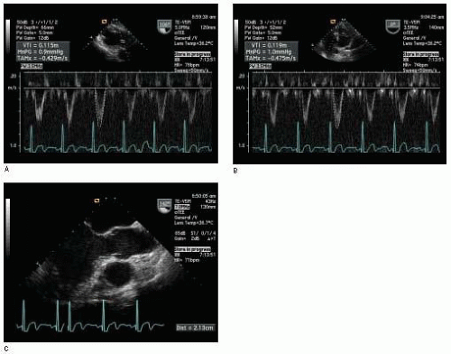
FIGURE 22.7. Data for LVOT stroke volume calculation. A: The VTILVOT can be measured using pulsed wave Doppler with the sample volume in the LVOT just proximal to the aortic valve from a transgastric long-axis view. B: Alternatively, the VTILVOT can be measured using pulsed wave Doppler with the sample volume in the LVOT just proximal to the aortic valve from a deep transgastric long-axis view. C: The diameter of the LVOT is usually measured from the midesophageal long-axis view of the aortic valve. VTI, velocity-time integral; LVOT, left ventricular outflow tract.

Alternatively, a cine of a “normal” aortic valve from the same midesophageal short-axis view is used to measure the side (S) in cm of the equilateral opening of the valve during midsystole. Several measurements may be made and then averaged in order to improve accuracy. The formula for the area of an equilateral triangle is then used to calculate the cross-sectional area of the aortic valve:

CSA AV (cm2) = 0.433 × (S)2


Data for Main PA Stroke Volume Calculation (Fig. 22.9)

The pulsed wave Doppler sample volume is placed in the main pulmonary artery using the upper esophageal short-axis view of the aortic arch (with the transducer rotated
from 80° to 90°) or the midesophageal short-axis view of the aorta for determination of the VTIPA. The diameter (cm) of the main pulmonary artery is obtained from either view at the same location for determination of the cross-sectional area using the formula for the area of a circle:

CSA PA (cm2) = 0.785 × DPA2


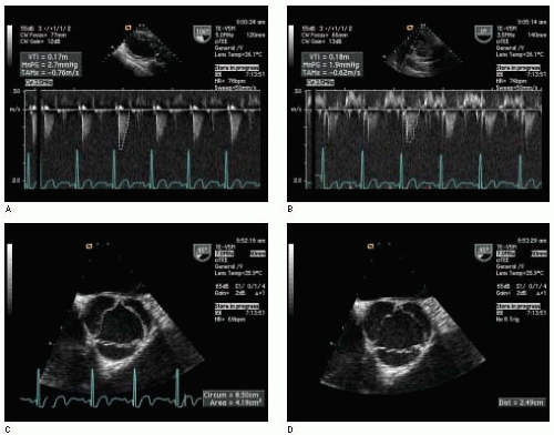
FIGURE 22.8. Data for transaortic valve stroke volume calculation. A: The VTIAV can be measured with the continuous wave Doppler beam placed through the aortic valve from a transgastric long-axis view. B: Alternatively, the VTIAV can be measured with the continuous wave Doppler beam placed through the aortic valve from a deep transgastric long-axis view. C: Planimetry can be used to measure the cross-sectional area of the aortic valve orifice during midsystole from a cine of the midesophageal short-axis view of the aortic valve. D: Alternatively, the length of a side of the aortic valve can be measured in midsystole for calculating the aortic valve area. VTI, velocity-time integral; AV, aortic valve; S, length of side of aortic valve.

In either case, fluctuation in the diameter of the main pulmonary artery during the cardiac cycle makes stroke volume measurement at this location less reliable than at the LVOT or aortic valve (12).


Data for RVOT Stroke Volume Calculation (Fig. 22.10)

The RVOT may be visualized using a transgastric RV inflow-outflow view with the transducer rotated from 110° to 150° and the probe turned to the right. The pulsed wave Doppler sample volume is placed in the RVOT just proximal to the pulmonic valve for determination of the VTIRVOT. The diameter (cm) of the RVOT is best obtained from the same view at the same location for determination of cross-sectional area, using the formula for the area of a circle:

CSARVOT (cm2) = 0.785 × DRVOT2


Alternatively, the diameter (cm) of the RVOT can be measured from the upperesophageal short-axis view of the aortic arch in some patients.


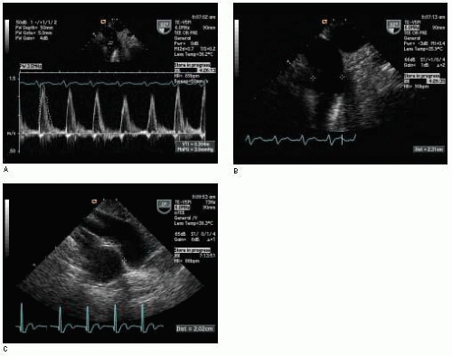
FIGURE 22.9. Data for main PA stroke volume calculation. A: The VTIPA can be measured using pulsed wave Doppler with the sample volume in the main pulmonary artery using the upperesophageal short-axis view of the aortic arch. B: The diameter of the main pulmonary artery can be measured from the same view at the same location. C: Alternatively, the diameter of the main pulmonary artery (as well as the VTIPA) can be measured using the midesophageal short-axis view of the ascending aorta (the VTIPA may also be obtained from this view). VTI, velocity-time integral; PA, pulmonary artery.


Data for Transmitral Stroke Volume Calculation (Fig. 22.11)

The pulsed wave Doppler sample volume is placed at the level of the mitral valve annulus, using the midesophageal four-chamber view (alternatively, the midesophageal two-chamber view or midesophageal long-axis view may be used) for determination of the VTIMV. While the mitral valve orifice is not truly elliptical during diastole, it is more elliptical than circular. The American Society of Echocardiography concluded in its document on quantitation of Doppler echocardiography that assumption of a circular orifice has generally worked well for all valves other than the tricuspid (13). Nevertheless, it may be preferable to estimate the cross-sectional area of the mitral valve, using the formula for an ellipse. The long and short diameters (cm) of the mitral valve annulus can be approximated using measurements from the midesophageal four-chamber and two-chamber views. The formula for an ellipse can then be used to calculate the cross-sectional area of the mitral valve:

CSA MV (cm2) = 0.785 × D1 × D2

The irregular semielliptical shape of the mitral valve orifice and the fluctuation in its size during diastole make stroke volume measurement at this location less reliable than at the LVOT or aortic valve (12).


DOPPLER MEASUREMENT OF PULMONARY-TO-SYSTEMIC FLOW RATIO (Qp/Qs)

The ratio of pulmonic-to-systemic blood flow, Qp/Qs usually indicates the magnitude of a shunt (i.e., atrial septal defect, ventricular septal defect, or patent pulmonary ductus arteriosus) and may be useful information in determining
the need for surgery or the timing of surgery. Qp/Qs can be calculated once the systemic stroke volume (measured at the LVOT or aortic valve) and pulmonic stroke volume (measured at the PA or RVOT) have been determined (14):


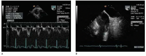
FIGURE 22.10. Data for RVOT stroke volume calculation. A: The VTIRVOT can be measured using pulsed wave Doppler with the sample volume placed just proximal to the pulmonic valve from a transgastric RV inflow-outflow view (transducer usually rotated from 110° to 150° and the probe turned to the right). B: The diameter of the RVOT may be obtained from this same view or the upper esophageal short-axis view of the aortic arch. VTI, velocity-time integral; RVOT, right ventricular outflow tract.

Qp/Qs = (SVPA × HR) / (SVLVOT × HR) Qp/Qs = SVPA / SVLVOT

Potential errors in the estimation of Qp/Qs are the same as for other Doppler determinations of stroke volume. It should be noted that there is also the possibility of compounding calculated Doppler stroke volume errors in the calculation of Qp/Qs with this formula (i.e., if SVPA is overestimated and SVLVOT is underestimated, then Qp/Qs may be significantly overestimated). This potential propagation of errors will lead to a range in the confidence intervals for Qp/Qs, which is unacceptable to many clinicians using TEE. Furthermore, in the presence of significant aortic regurgitation this calculation is not accurate and Qp/Qs will be underestimated.


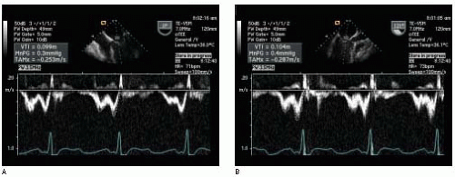
FIGURE 22.11. Data for transmitral stroke volume calculation. The VTIMV can be measured using pulsed wave Doppler with the sample volume placed within the mitral valve annulus using any midesophageal view of the mitral valve. A: The VTIMV measured from the midesophageal four-chamber view. B: The VTIMV measured from the midesophageal long-axis view in the same patient. (continued)


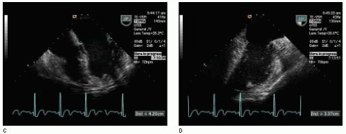
FIGURE 22.11. (Continued) C: The long diameter (D1) of the mitral valve annulus can be approximated using measurements from the midesophageal four-chamber view. D: The short diameter (D2) of the mitral valve annulus can be approximated using measurements from the midesophageal two-chamber view. VTI, velocity-time integral; MV, mitral valve.


DOPPLER MEASUREMENT OF REGURGITANT VOLUME AND FRACTION


Volumetric Method (Fig. 22.12)

Regurgitant volume (RV) is the volume of blood that flows backwards through a regurgitant valve during one cardiac cycle. Conservation of mass says that the stroke volume delivered to the systemic circulation (SVSYSTEMIC) must equal the total forward stroke volume across a regurgitant valve (SVTOTAL) minus the regurgitant volume:

SVSYSTEMIC = SVTOTAL − RV

Thus, regurgitant volume can be calculated once SVTOTAL and SVSYSTEMIC have been determined:

RV = SVTOTAL − SVSYSTEMIC

The regurgitant fraction (RF) for any valve is calculated as the ratio of regurgitant volume to total forward flow across the regurgitant valve expressed as a percentage.

RF (%) = (RV / SVTOTAL) × 100%


Assessment of Mitral Regurgitation (Fig. 22.13)

In mitral regurgitation, the SVTOTAL is the mitral inflow stroke volume and the SVSYSTEMIC is the LVOT stroke volume. Thus, the mitral valve regurgitant volume can be estimated by subtracting the LVOT stroke volume from the mitral valve inflow stroke volume and then the mitral regurgitant fraction can be calculated (15):

RVMV = SVMVI − SVLVOT RFMV (%) = (RVMV / SVMVI) × 100%

This method of assessing mitral regurgitation is performed infrequently during TEE examinations due to the time required to acquire the data and the possibility of compounding calculated Doppler stroke volume errors during the calculation of mitral regurgitant volume or
fraction. This potential propagation of errors will lead to a range in the confidence intervals for the mitral valve regurgitant volume, which is unacceptable to many clinicians. A particular problem exists with reliably measuring the mitral valve inflow stroke volume due to the irregular shape of the mitral valve orifice (semielliptical) and the fluctuation in its size during diastole (12). Furthermore, in the presence of significant aortic regurgitation this calculation is not accurate and mitral regurgitant volume will be underestimated.


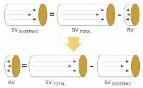
FIGURE 22.12. The volumetric method for calculation of regurgitant volume. Conservation of mass dictates that regurgitant volume must be equal to the difference between the total forward stroke volume across the regurgitant valve and the systemically delivered stroke volume. RV, regurgitant volume; SVTOTAL, total forward stroke volume across the regurgitant valve; SVSYSTEMIC, systemically delivered stroke volume.


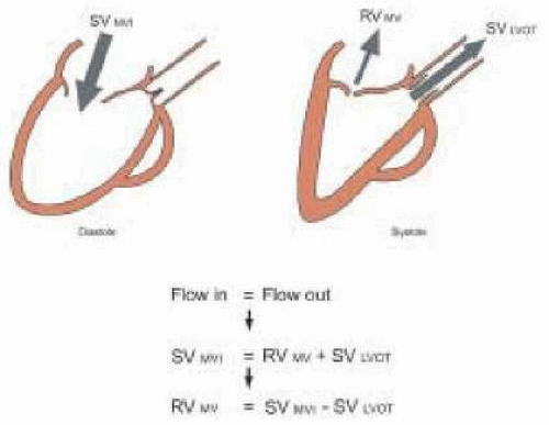
FIGURE 22.13. Assessment of mitral regurgitant volume using the volumetric method. Diastolic flow into the left ventricle must equal systolic flow out. Therefore, the mitral regurgitant volume must equal the difference between the mitral valve inflow stroke volume and the LVOT stroke volume. This method will underestimate mitral regurgitant volume in the presence of significant aortic regurgitation. RVMV, mitral regurgitant volume; SVMVI, mitral valve inflow stroke volume; SVLVOT, left ventricular outflow tract stroke volume.


Assessment of Aortic Regurgitation (Fig. 22.14)

In aortic regurgitation, the SVTOTAL is the LVOT forward stroke volume and the SVSYSTEMIC is the mitral valve inflow stroke volume. Thus, the aortic valve regurgitant volume can be estimated by subtracting the mitral valve inflow stroke volume from the LVOT forward stroke volume and then aortic regurgitant fraction can be calculated (15):

RVAV = SVLVOT − SVMVI

RFAV (%) = (RVAV / SVLVOT) × 100%

This method of assessing aortic regurgitation is also performed infrequently during TEE examinations due to the time required to acquire the data and the possibility of compounding calculated Doppler stroke volume errors during the calculation of aortic regurgitant volume or fraction. This potential propagation of errors will lead to a range in the confidence intervals for the aortic valve regurgitant volume that is unacceptable to many clinicians. A particular problem exists with reliably measuring the mitral valve inflow stroke volume due to the irregular semielliptical shape of the mitral valve orifice and the fluctuation in its size during diastole (12). Furthermore, in the presence of significant mitral regurgitation this calculation is not accurate and aortic regurgitant volume will be underestimated.


FIGURE 22.14. Assessment of aortic regurgitant volume using the volumetric method. Diastolic flow into the left ventricle must equal systolic flow out. Therefore, the aortic regurgitant volume must be equal to the difference between the LVOT stroke volume and the mitral valve inflow stroke volume. This method will underestimate aortic regurgitant volume in the presence of significant mitral regurgitation. RVAV, aortic regurgitant volume; SVLVOT, left ventricular outflow tract stroke volume; SVMVI, mitral valve inflow stroke volume.


Proximal Convergence Method

As blood flows towards a regurgitant orifice (i.e., mitral regurgitation), or in some cases a stenotic orifice (i.e., mitral stenosis), blood flow velocity increases with the formation of multiple concentric “isovelocity” shells (Fig. 22.15) (16,17). These “isovelocity” shells can be “seen” with color flow imaging, as seen in Fig. 22.16, and have been termed proximal isovelocity surface areas (PISAs). The size of a PISA proximal to a regurgitant orifice can be altered by adjusting the Nyquist limit of the color flow map. As the negative aliasing velocity is reduced (in the case of mitral regurgitation), the transition from red to blue will occur farther from the regurgitant orifice resulting in a hemispheric shell with a larger radius (r). The instantaneous velocity of blood at the PISA is the same as the aliasing velocity on the color flow map. The instantaneous flow rate through a PISA that is a hemispheric shell is equal to the product of the area of the PISA and the instantaneous velocity of blood at the PISA:

Only gold members can continue reading. Log In or Register to continue

Stay updated, free articles. Join our Telegram channel

Jul 15, 2016 | Posted by in CARDIOLOGY | Comments Off on Assessment of Perioperative Hemodynamics

Full access? Get Clinical Tree

Get Clinical Tree app for offline access